Inequality of opportunity
Methodological details
In a nutshell
Inequality of opportunity (IOp) is the part of overall inequality that stems from factors beyond individual control such as gender, race, or family background. These predetermined characteristics are called circumstances. IOp measurement follows a two-step procedure:
- The distribution of the outcome of interest is transformed into a counterfactual distribution which reflects only and fully the unfair inequality in the outcome, while all the fair inequality is removed.
Ex: Replace individual income by the average income of all individuals that share the same circumstances. - A measure of inequality is applied to the counterfactual distribution.
Ex: The Gini index or the mean logarithmic deviation (MLD).
The main challenge is to determine the most appropriate partition of the population into groups of individuals sharing the same circumstances. With too few groups, most inequality attributable to circumstances will go undetected and IOp estimates will suffer from a downward bias. With too many, the model will overfit the data generating an upward bias (Brunori et al. 2019).
We overcome this challenge using a suite of tree-based machine learning algorithms, which select optimal partitions without imposing prior specifications. We implement this approach on 196 household surveys selected to balance coverage and comparability. This allows us to compute IOp estimates for 72 countries, over a period of up to 44 years (Ferreira et al. 2026).
Minimalist example
Consider a population of 50 individuals whose outcomes are fully determined by their relative effort and the following circumstances.
- Place of birth: Rural or Urban
- Ethnicity: Minority or Majority
These circumstances partition the population into 4 types: rural minority, rural majority, urban majority, and urban minority. The real-world counterpart of this step is much less straightforward since there are considerably more categories to consider. This is where we use machine learning to determine the most relevant type partition.
The figure below represents each of the 50 individuals with a brick colored according to their type, and placed on the horizontal axis according to their outcome value, from 1 to 11. Overall inequality is computed over this distribution using the Gini index or the mean logarithmic deviation, for instance.
Inequality of opportunity (IOp) aims to isolate the part of overall inequality that stems from circumstances rather than effort. To this end, this distribution is transformed by assigning every individual the average outcome of their type, as illustrated on the figure above. Inequality of opportunity is computed over this distribution using the Gini index or the mean logarithmic deviation, for instance.
By construction, IOp is lower than overall inequality. These two measures are comparable, such that IOp can be expressed as a fraction of overall inequality, called relative IOp. In the example above, 0.125 / 0.224 = 56% of overall inequality is explained by circumstances.
The structure of inequality of opportunity underlying a given estimate can be represented in several ways. The figure below represents each type with a bar, sorted by ascending order of average outcome along the horizontal axis. The width of each bar is proportional to the corresponding type’s share in the population, and its height to their average outcome relative to that of the overall population. The figure on the right is a tree representation of the underlying partition of the population into the four possible types.
Concepts of inequality of opportunity
Measuring inequality of opportunity relies on the construction of a counterfactual distribution that isolates inequality driven by predetermined circumstances. Different versions of the counterfactual distribution can be considered. They express different and sometimes conflicting views on equality of opportunity, and the way they rank distributions can differ (see Ferreira and Peragine (2016) for a discussion). We use ex-ante IOp as our headline estimates, and also provide ex-post IOp estimates in the augmented dataset (see Download section of the website).
Ex-ante IOp considers that opportunity sets available to individuals should have the same expected value regardless of circumstances (Van de Gaer 1993). Consider a partition of the population into groups of individuals that share the same circumstances, called types. Ex-ante IOp consists in computing inequality on a counterfactual distribution that is obtained by replacing each individual outcome by the average outcome of the type to which the individual belongs. This smoothing transformation removes all inequality within types.
Ex-post IOp considers that individuals exerting the same degree of effort should achieve the same outcome (Roemer 1998). Consider a partition of the population into groups of individuals that belong to the same quantile in their respective type distributions. These groups are called tranches, and capture the relative degree of effort. Ex-post IOp consists in computing inequality on a counterfactual distribution that is obtained by replacing individual outcomes in each tranche with the ratio between that outcome and the average outcome of the tranche.
Counterfactual distribution estimation
The estimation of a counterfactual distribution to isolate the unfair inequality in an outcome is a key step of IOp measurement. The fact that estimation typically occurs in samples rather than entire populations gives rise to a tradeoff between two different kinds of bias in selecting a prediction model to construct the counterfactual distribution. With too few variables and interactions, most inequality attributable to circumstances will go undetected and IOp estimates will suffer from a downward bias. With too many, the model will overfit the data generating an upward bias (Brunori et al. 2019).
Different prediction methods have been used in the past but, until recently, these generally relied on arbitrary or ad hoc specifications. In addition, constraining all countries to a given pre-specified model would not be appropriate as the set of relevant circumstances is likely to be context-dependent. We address these challenges using a suite of data-driven tree-based supervised machine learning techniques to select optimal prediction models.
Tree-based data-driven approach
Data-driven machine learning approaches, which select optimal partitions without imposing prior specifications, are naturally suited to the estimation of IOp from survey data. Tree-based methods, in particular, offer three main advantages.
- They partition the regressor space into non-overlapping regions, assigning individuals to mutually exclusive groups defined by the interaction of their circumstances. This is directly consistent with the notion of types having access to different sets of opportunities.
- The possibility to tune the algorithm prevents the model from becoming too complex and overfitting the data (Chakravarty and Eichhorn (1994), Brunori et al. (2019)), while maximizing out of sample predictive power to minimize the downward bias frequently highlighted by researchers (Ferreira and Gignoux 2011).
- Unlike standard recursive partitioning algorithms, trees do not tend to overuse variables with many distinct values as splitting variables, ensuring that the selection of circumstances is driven by statistical significance rather than the number of categories (Hothorn et al. 2006).
Application to both concepts of IOp
For ex-ante IOp, we partition the population into types using a Conditional Inference Tree (Ctree) algorithm, which searches for the partition that maximizes the statistical significance of differences in average outcome between subsamples (Hothorn et al. 2006). It is therefore especially well-suited for ex-ante IOp, which, as discussed above, uses type means to construct the counterfactual distribution. For ex-post IOp, we follow Brunori et al. (2026) and use Transformation Trees (Trafotrees), which are analogous to Ctrees, but partition the population using the full conditional distribution of the outcome rather than only its mean, which is better suited to this concept (Hothorn and Zeileis 2021).
Although single trees are low-bias estimators, they are known to have high variance, meaning that small changes in the data could lead to different partitions and unstable estimates. By aggregating predictions across many trees grown on different subsamples of the data, random forests substantially reduce variance while preserving the low bias of individual trees. Hence, we use conditional inference random forests instead of conditional inference trees to compute our headline estimates of ex-ante IOp (Hothorn et al. (2006), Brunori et al. (2023)). We are not aware of suitable methods to produce forests of Trafotrees that could be used for ex-post IOp (see Brunori et al. (2026) for a discussion).
We briefly describe the conditional inference tree, random forest, and transformation tree algorithms in the section Estimation details below (see also Brunori et al. (2023) and Brunori et al. (2026)).
Choice of summary measure
Once the counterfactual distribution \(\tilde{x}\) of outcome \(x\) has been obtained, an inequality index \(I(.)\) is used to obtain a scalar estimate of inequality of opportunity. The Gini index and the Mean logarithmic deviation (MLD) are most common in the literature and we align with this practice. We report the Gini as our headline measure because it is more sensitive to the central part of the distribution, where most of the between-type inequality occurs, whereas the MLD is more sensitive to the tails.
Two closely related versions of the IOp index can then be considered. The first one is the absolute measure of inequality of opportunity \(\text{IO}_\text{A} =I(\tilde{x})\). The second one is its relative counterpart, the ratio of \(\text{IO}_\text{A}\) to overall inequality: \[ \text{IO}_\text{R}=\frac{I(\tilde{x})}{I(x)} \]
\(\text{IO}_\text{R}\) can be interpreted as the share of total inequality that can be predicted by circumstances, i.e., by inherited characteristics which people cannot be held responsible for.
Data sources
Sample definitions
We gather data from 72 countries, drawn from 196 household surveys selected balancing two key desiderata: broad country coverage and methodological comparability. We restrict our attention to household surveys because administrative data on social security records across generations are not available in most countries. Surveys were selected according to four criteria.
- The sample has to be representative of the entire country.
- It must contain information on a money-metric wellbeing indicator, either income or consumption expenditure, at the individual or household level.
- It has to contain individual-level information on at least five of the following seven circumstance variables: area or region of birth, sex, ethnicity, occupation of the father and/or mother, and education of the father and/or mother.
- The last criterion is a minimum of 1,500 individual observations with complete information and strictly positive outcomes. All samples are restricted to individuals aged 18 or older.
Details of all countries, time periods, and surveys are provided in the table below.
Data sources table
| Country | Year(s) covered | Survey and acronym | Research team |
|---|---|---|---|
| Argentina | 2014 | Encuesta Nacional sobre la Estructura Social (ENES) | CEDLAS |
| Armenia | 2016 | Life in Transition Survey (LITS) | ADB & Monash |
| Australia | 2005, 2007, 2009, 2011, 2013, 2015, 2017, 2019 | Household, Income and Labour Dynamics in Australia (HILDA) | ADB & Monash |
| Austria | 2005, 2011, 2019 | European Union Statistics on Income and Living Conditions (EU-SILC) | LSE |
| Belgium | 2005, 2011, 2019 | European Union Statistics on Income and Living Conditions (EU-SILC) | LSE |
| Benin | 2018 | Enquête Harmonisée sur les Conditions de Vie des Ménages (EHCVM) | Bari |
| Bolivia | 2008 | Encuesta de Hogares (EH) | CEDLAS |
| Brazil | 2014 | Pesquisa Nacional por Amostra de Domicilios Contínua Anual (PNAD) | CEDLAS |
| Bulgaria | 2011, 2019 | European Union Statistics on Income and Living Conditions (EU-SILC) | LSE |
| Burkina Faso | 2018 | Enquête Harmonisée sur les Conditions de Vie des Ménages (EHCVM) | Bari |
| Chile | 2006, 2011, 2013, 2015 | Encuesta de Caracterización Socioeconómica Nacional (CASEN) | CEDLAS |
| China | 2010, 2012, 2014, 2016, 2018 | China Family Panel Studies (CFPS) | LSE |
| Colombia | 2010 | Encuesta Nacional de Calidad de Vida (ENCV) | CEDLAS |
| Croatia | 2011 | European Union Statistics on Income and Living Conditions (EU-SILC) | LSE |
| Cyprus | 2005, 2011, 2019 | European Union Statistics on Income and Living Conditions (EU-SILC) | LSE |
| Czech Republic | 2005, 2011, 2019 | European Union Statistics on Income and Living Conditions (EU-SILC) | LSE |
| Denmark | 2005, 2011, 2019 | European Union Statistics on Income and Living Conditions (EU-SILC) | LSE |
| Ecuador | 2006, 2014 | Encuesta Condiciones de Vida (ECV) | CEDLAS |
| Estonia | 2005, 2011, 2019 | European Union Statistics on Income and Living Conditions (EU-SILC) | LSE |
| Finland | 2005, 2011, 2019 | European Union Statistics on Income and Living Conditions (EU-SILC) | LSE |
| France | 2005, 2011, 2019 | European Union Statistics on Income and Living Conditions (EU-SILC) | LSE |
| Gambia | 2015 | Integrated Household Survey (IHS) | Bari |
| Georgia | 2016 | Life in Transition Survey (LITS) | ADB & Monash |
| Germany | 2005, 2011, 2019 | European Union Statistics on Income and Living Conditions (EU-SILC) | LSE |
| Ghana | 2013, 2017 | Ghana Living Standard Survey (GLSS) | Bari |
| Greece | 2005, 2011, 2019 | European Union Statistics on Income and Living Conditions (EU-SILC) | LSE |
| Guatemala | 2000, 2006, 2011 | Encuesta Nacional sobre Condiciones de Vida (ENCOVI) | CEDLAS |
| Guinea Bissau | 2018 | Enquête Harmonisée sur les Conditions de Vie des Ménages (EHCVM) | Bari |
| Hungary | 2005, 2011, 2019 | European Union Statistics on Income and Living Conditions (EU-SILC) | LSE |
| Iceland | 2005 | European Union Statistics on Income and Living Conditions (EU-SILC) | LSE |
| India | 2005, 2012 | India Human Development Survey (IHDS) | ADB & Monash |
| Indonesia | 2000, 2014 | Indonesian Family Life Survey (IFLS) | ADB & Monash |
| Ireland | 2005, 2011, 2019 | European Union Statistics on Income and Living Conditions (EU-SILC) | LSE |
| Italy | 2005, 2011, 2019 | European Union Statistics on Income and Living Conditions (EU-SILC) | LSE |
| Ivory Coast | 2018 | Enquête Harmonisée sur les Conditions de Vie des Ménages (EHCVM) | Bari |
| Kazakhstan | 2016 | Life in Transition Survey (LITS) | ADB & Monash |
| Kyrgyzstan | 2016 | Life in Transition Survey (LITS) | ADB & Monash |
| Latvia | 2005, 2011, 2019 | European Union Statistics on Income and Living Conditions (EU-SILC) | LSE |
| Lithuania | 2005, 2011, 2019 | European Union Statistics on Income and Living Conditions (EU-SILC) | LSE |
| Luxembourg | 2005, 2011, 2019 | European Union Statistics on Income and Living Conditions (EU-SILC) | LSE |
| Malawi | 2020 | Malawi Fifth Integrated Household Survey (MFIHS) | Bari |
| Mali | 2019 | Enquête Harmonisée sur les Conditions de Vie des Ménages (EHCVM) | Bari |
| Malta | 2011, 2019 | European Union Statistics on Income and Living Conditions (EU-SILC) | LSE |
| Mexico | 2017 | Encuesta de Movilidad Social (EMOVI) | Provided by CEEY |
| Mongolia | 2016 | Life in Transition Survey (LITS) | ADB & Monash |
| Nepal | 2003, 2011 | Nepal Living Standards Survey (NLSS) | ADB & Monash |
| Netherlands | 2005, 2011, 2019 | European Union Statistics on Income and Living Conditions (EU-SILC) | LSE |
| Niger | 2018 | Enquête Harmonisée sur les Conditions de Vie des Ménages (EHCVM) | Bari |
| Nigeria | 2019 | Nigeria Living Standards Survey (NLSS) | Bari |
| Norway | 2005, 2011, 2019 | European Union Statistics on Income and Living Conditions (EU-SILC) | LSE |
| Panama | 2003 | Encuesta de Niveles de Vida (ENV) | CEDLAS |
| Peru | 2001, 2006, 2007, 2008, 2009, 2010, 2011, 2012, 2013, 2014, 2015 | Encuesta Nacional de Hogares sobre Condiciones de Vida y Pobreza (ENAHO) | CEDLAS |
| Poland | 2005, 2011, 2019 | European Union Statistics on Income and Living Conditions (EU-SILC) | LSE |
| Portugal | 2005, 2011, 2019 | European Union Statistics on Income and Living Conditions (EU-SILC) | LSE |
| Romania | 2011, 2019 | European Union Statistics on Income and Living Conditions (EU-SILC) | LSE |
| Senegal | 2018 | Enquête Harmonisée sur les Conditions de Vie des Ménages (EHCVM) | Bari |
| Sierra Leone | 2011, 2018 | Sierra Leone Integrated Household Survey (SLIHS) | Bari |
| Slovakia | 2005, 2011, 2019 | European Union Statistics on Income and Living Conditions (EU-SILC) | LSE |
| Slovenia | 2005, 2011, 2019 | European Union Statistics on Income and Living Conditions (EU-SILC) | LSE |
| South Africa | 2008, 2012, 2015, 2017 | National Income Dynamics Study (NIDS) | LSE |
| South Korea | 1999, 2001, 2003, 2005, 2007, 2009, 2011, 2013, 2015, 2017, 2019 | Korean Labour and Income Panel Study (KLIPS) | ADB & Monash |
| Spain | 2005, 2011, 2019 | European Union Statistics on Income and Living Conditions (EU-SILC) | LSE |
| Sweden | 2019 | European Union Statistics on Income and Living Conditions (EU-SILC) | LSE |
| Switzerland | 2011, 2019 | European Union Statistics on Income and Living Conditions (EU-SILC) | LSE |
| Tajikistan | 2016 | Life in Transition Survey (LITS) | ADB & Monash |
| Tanzania | 2009, 2011, 2013 | National Panel Survey (NPS) | Bari |
| Timor-Leste | 2007, 2014 | Timor-Leste Survey of Living Standards (TSLS) | ADB & Monash |
| Togo | 2018 | Enquête Harmonisée sur les Conditions de Vie des Ménages (EHCVM) | Bari |
| Uganda | 2010, 2011, 2012, 2014 | National Panel Survey (NPS) | Bari |
| UK | 2005, 2011 | European Union Statistics on Income and Living Conditions (EU-SILC) | LSE |
| USA | 1970, 1972, 1974, 1976, 1978, 1980, 1982, 1984, 1986, 1988, 1990, 1992, 1994, 1996, 1998, 2000, 2002, 2004, 2006, 2008, 2010, 2012, 2014 | Panel Study of Income Dynamics (PSID) | LSE |
| Uzbekistan | 2016 | Life in Transition Survey (LITS) | ADB & Monash |
Time coverage varies significantly across countries, from a single survey-year for some, such as Armenia (2016), Colombia (2010), or Mali (2019), to eight or more years for others, such as the United States, Peru, or Australia. Coverage is broad for Europe, North America, South Asia, Latin America and Caribbean, and East Asia and Pacific, each representing more than 65% of their regional population, but it remains limited for the Middle East and North Africa (0.1%). In total, we cover 72 out of 217 countries, representing 66.9% of the world’s population in 2022.
| Geographical Macro Regions | Number of countries (World Bank) | Number of countries (This study) | Share of countries (%) | Share of population (%) |
|---|---|---|---|---|
| East Asia & Pacific | 37 | 6 | 16.22 | 75.26 |
| Europe & Central Asia | 58 | 36 | 62.07 | 65.96 |
| Latin America & Caribbean | 42 | 10 | 23.81 | 82.9 |
| Middle East & North Africa | 21 | 1 | 4.76 | 0.11 |
| North Americaa | 3 | 1 | 33.33 | 89.53 |
| South Asia | 8 | 2 | 25 | 75.43 |
| Sub-Saharan Africa | 48 | 16 | 33.33 | 49.34 |
| Total | 217 | 72 | 33.18 | 66.89 |
| Economic Macro Regions | Number of countries (World Bank) | Number of countries (This study) | Share of countries (%) | Share of population (%) |
|---|---|---|---|---|
| High Income | 83 | 35 | 42.17 | 77.4 |
| Upper-middle Income | 54 | 14 | 25.93 | 82.26 |
| Lower-middle Income | 54 | 14 | 25.93 | 59.36 |
| Low Income | 26 | 9 | 34.62 | 22.93 |
| Total | 217 | 72 | 33.18 | 66.89 |
a Mexico is included in Latin America and Caribbean. North America includes Canada, the United States and Bermuda.
Variable definitions
The outcome variable is equivalized household disposable income, i.e., total household income divided by the square root of household size to account for economies of scale, measured at the individual level. Where income data is unavailable, we use equivalized household consumption expenditure instead. This measure ignores intra-household inequality by construction, which mechanically reduces the importance of the sex circumstance variable.
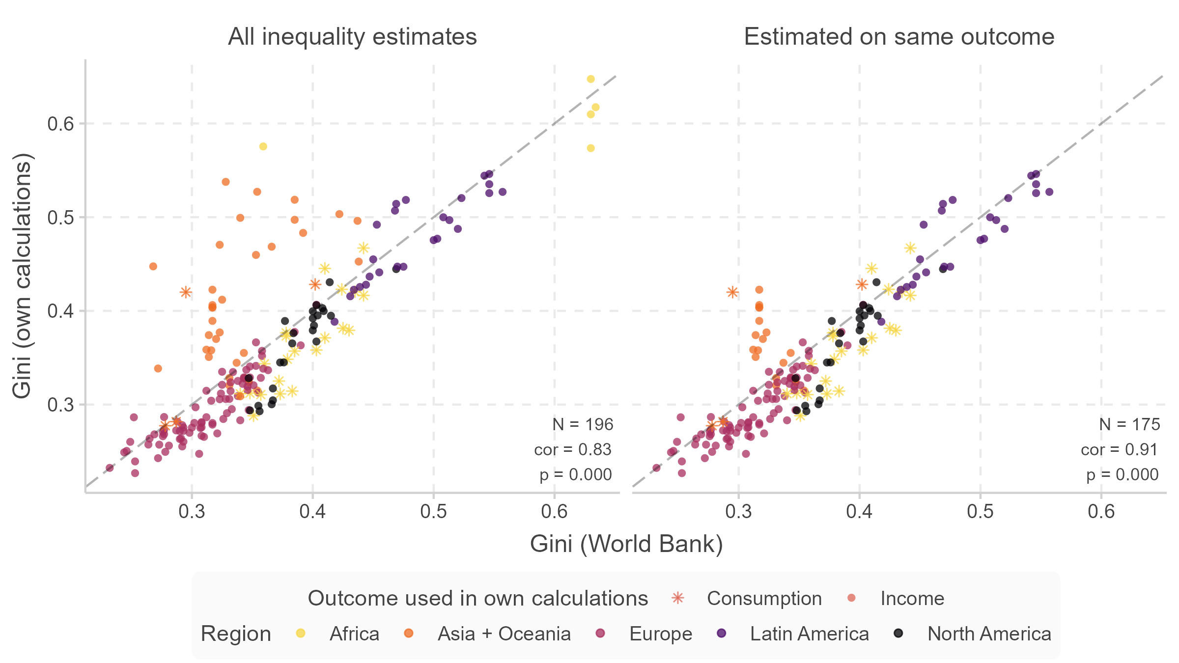
Before estimation we adjust equivalized household income (or consumption) by subtracting the contribution of age and age squared in a regression approach to control for systematic correlations between life cycle and the outcome distribution (Solon 1992). For comparability purposes, all monetary values are expressed in 2017 US dollars after adjusting by Purchasing Power Parity (PPP) and the Consumer Price Index (CPI). Both adjustments are described in Estimation details > Variable adjustments, along with additional details. The use of an equivalence scale, the age adjustment, and our sample restrictions, may generate slightly different inequality indices from those available in other compilations. The Figure below plots our estimates of the Gini index of income inequality against those published by the World Bank (World Development Indicators). The two measures are highly correlated (\(\rho\) = 0.91), and results show relatively little deviation from the 45-degree line.
As regards the circumstance variables, all are categorical in nature and the definition of categories is inevitably specific to each country. To reduce computational cost, categorical variables are limited to a maximum of 25 values. If a circumstance variable has 26 or more categories, they are merged until 25 different values are reached. Any threat to comparability posed by these country idiosyncrasies is substantially mitigated by the data-driven nature of the algorithms we use to partition the sample.
Estimation details
Ex-ante Inequality of Opportunity
To partition the population into types with the ex-ante approach to estimating IOp, we follow Brunori et al. (2023) in using conditional inference regression trees (Ctrees) and conditional inference random forests (CForest) developed by Hothorn et al. (2006).
The Ctree algorithm
The core challenge in measuring inequality of opportunity is deciding how to divide the population into types. If we observed the entire population, we could simply group everyone who shares identical circumstances together. In practice, we work with samples, so we need a principled method that finds the most meaningful partition without over-fitting to the data at hand. Ctrees provide exactly this: a supervised machine-learning algorithm that recursively splits the sample on circumstances, stopping only when further splits are no longer statistically justified.
Concretely, the algorithm proceeds as follows:
- Set a confidence level \((1 - \alpha)\). This controls how strong the statistical evidence needs to be before making a split — a lower \(\alpha\) means stricter requirements.
- Test the association between the outcome and each circumstance. If the Bonferroni-corrected p-value of every test exceeds \(\alpha\), stop — no circumstance is informative enough to justify a further split. Otherwise, continue.
- Select the circumstance with the smallest adjusted p-value as the splitting variable \(c\) — the circumstance most strongly associated with differences in outcomes.
- Among all possible binary partitions of the sample based on \(c\), compute the p-value for the null hypothesis that the means in the two sub-samples are equal.
- Choose the partition with the smallest p-value — the split that creates the two groups whose average outcomes differ most.
- Repeat steps 2–5 for each resulting node until no further split is statistically justified in any sub-sample.
The result is a partition of the population into types \(t = \{1, \ldots, T\}\), each defined by a specific combination of circumstances. For each type we compute the population-weighted share \(\hat{w}_t\) and the weighted mean outcome \(\hat{\mu}_t\).
How is ex-ante IOp calculated from this? We construct a counterfactual distribution in which every person receives the average outcome of their type — erasing within-type inequality and keeping only the inequality between types. Formally, we replace the outcome of individual \(i\) in type \(t\) with \(\tilde{y}_{i,t} = \hat{\mu}_t\), and measure inequality in this counterfactual distribution \(\tilde{y}\):
\[\widehat{IOp}_a = I(\tilde{y})\]
We use the Gini coefficient as the inequality measure \(I(\cdot)\) for our headline estimates, but we also provide estimates obtained using the mean logarithmic deviation (MLD) in the augmented dataset (see Download section of the website).
The figure below shows an example Ctree. Each terminal node displays the expected outcome of that type, normalized by the sample mean — so a value above 1 indicates an above-average outcome. The first split is on ethnicity, then on education level within each ethnic group.
Algorithm specificities
We follow econometric convention and set \(\alpha\) = 0.01, meaning a split is made only when the statistical evidence is strong (99% confidence).
Each terminal node must contain at least 1% of sample observations (or 50, if the sample size is below 5,000). This floor prevents the tree from creating types so small that they are meaningless or driven by noise, and limits the influence of varying sample sizes across countries.
For robustness, a second tree is estimated relaxing the minimum to 0.1%. If the resulting partition differs, both plots are stored for inspection.
Sampling weights are not used to determine splits. Including them would artificially inflate the effective sample size — effectively treating each observation as many identical copies — causing the tree to grow excessively deep and split on statistically trivial differences. Weights are used to compute the counterfactual distribution and the final IOp estimate.
All remaining parameters follow the defaults of the ctree function in the R package partykit (Hothorn et al. 2023).
Limitations and interpretation
Regression trees are characterized by low bias but high variance (Hastie et al. 2009). In plain terms: a tree will correctly identify the structure of opportunity in the data it sees, but that structure can look somewhat different if we had drawn a slightly different sample from the same population. This is not a flaw unique to Ctrees — it is a fundamental property of all tree-based methods.
This has two practical implications:
- Do not over-interpret the exact structure of a single tree. The precise splits shown may not hold in a different dataset from the same country.
- Always check population shares alongside the tree structure. A terminal node may represent a tiny fraction of the population, meaning its apparent characteristics may be driven by just a handful of observations and should not be generalized.
The example below illustrates why this matters.
Imagine a country with three ethnic groups A, B and C. Groups A and B are poor minorities living mostly in rural areas with similar average incomes; group C is a privileged urban group. In a sample of 1,000, group C makes up 80% of city-dwellers, group B makes up 19.9%, and group A is represented by just one person.
Now suppose that one person from group A happens to have an unusually high income. The Ctree may then group A together with C — making A appear privileged — rather than with B, where it truly belongs. This is not a mistake in the algorithm; it is simply following the data it has been given.
The figure below shows what this misclassified tree looks like, followed by the type-composition table that reveals the truth: a member of group A has a 99% probability of belonging to the worst-off type.
| Ex. Outcome | A | B | C | Population share | |
|---|---|---|---|---|---|
| Ex. Outcome | 0.80 | 0.82 | 1.50 | ||
| Type 1 | 0.8 | 32.4% | 32.5% | 0.0% | 64.9% |
| Type 3 | 0.86 | 0.0% | 15.1% | 0.0% | 15.1% |
| Type 4 | 1.5 | 0.1% | 0.0% | 19.9% | 20.0% |
| Population share | 32.5% | 47.6% | 19.9% | 100.0% |
Ex-ante IOp using forests (CForest)
Because single trees have high variance, our preferred IOp estimate uses a Conditional inference random forest (CForest) (Breiman 2001; Hothorn et al. 2006).
The intuition is simple: instead of relying on one tree grown from one sample, a random forest grows many trees — each on a slightly different random sub-sample of the data — and aggregates their predictions. The result is far more stable: quirks of any single sample get averaged out across hundreds of trees, and the estimate of IOp becomes much less sensitive to which particular individuals happened to be surveyed.
Formally, a random forest draws different sub-samples of the original data and fits a Ctree to each one. Under the appropriate aggregation procedure, this process generates robust IOp estimates (Brunori et al. 2023).
For this reason, cross-country and over-time comparisons of ex-ante IOp in GEOM are always based on CForest results. Single Ctrees are shown alongside to give an interpretable picture of the opportunity structure, but the headline ex-ante IOp numbers come from the forest.
Key tuning parameters for the CForest:
- \(\alpha\) = 1 (mincriterion = 0): each individual tree is free to grow as deep as the data allow, with no significance threshold for splits. This intentional overfitting at the individual tree level is corrected for by the averaging across trees.
- Sub-sample share per iteration: the default 0.632 of the full sample.
- Minimum terminal node size: 0.1% of the sample (or 10, if the sample is below 1,000), to maximize comparability across surveys with different sample sizes.
- All other parameters follow the defaults of the
cforestfunction in partykit (Hothorn et al. 2023).
Ex-post Inequality of Opportunity
To partition the population into types with the ex-post approach to estimating IOp, we follow Brunori et al. (2026) in using Transformation Trees (Trafotrees) introduced by Hothorn and Zeileis (2021).
Where the ex-ante approach asks whether people born into different circumstances end up with different expected outcomes, the ex-post approach goes further: it asks whether people who exert the same relative effort end up with different outcomes depending on their circumstances. In other words, it compares people who occupy the same rank within their own type-specific distribution.
The Trafotree algorithm
Trafotrees are closely analogous to Ctrees, with one key difference: instead of testing whether two sub-groups have different average outcomes, they test whether two sub-groups have different entire outcome distributions. This makes them especially suited to the ex-post question, where we care about differences across the full distribution — not only at the mean.
Concretely, the algorithm proceeds as follows:
- Set a confidence level \((1 - \alpha)\). This controls how strong the statistical evidence needs to be before making a split — a lower \(\alpha\) means stricter requirements.
- Set a Bernstein polynomial order \(m\). This determines how flexibly the algorithm can approximate the outcome distribution.
- Approximate the unconditional outcome distribution using a Bernstein polynomial of order \(m\). This produces \(m + 1\) parameters describing the shape of the distribution.
- Test the association between the outcome distribution and each circumstance using an m-fluctuation test. If the Bonferroni-corrected p-value of every test exceeds \(\alpha\), stop — no circumstance is informative enough to justify a further split. Otherwise, continue.
- Select the circumstance with the smallest adjusted p-value as the splitting variable \(c\) — the circumstance most strongly associated with differences in the outcome distribution.
- Among all possible binary partitions of the sample based on \(c\), compute the p-value for the null hypothesis that the two sub-sample distributions are equal.
- Choose the partition with the smallest p-value — the split that creates the two groups whose outcome distributions differ most.
- Repeat steps 3–7 for each resulting node until no further split is statistically justified in any sub-sample.
The result is a partition of the population into types \(t = \{1, \ldots, T\}\), each defined by a specific combination of circumstances. For each type, the algorithm estimates a parametric approximation of the full cumulative distribution function (CDF) — a richer output than the Ctree, which stores only the type mean.
How is ex-post IOp calculated from this? We construct a counterfactual distribution in which every person’s outcome is standardized by the average outcome of those at the same effort rank. Formally, for individual \(i\) at quantile \(q\) of their type-specific distribution, we replace the predicted outcome \(\hat{y}_{i,q}\) with:
\[ \tilde{y}_{i,q} = \frac{\hat{\mu}}{\hat{\mu}_q}\hat{y}_{i,q} \]
where \(\hat{\mu}\) is the overall population mean and \(\hat{\mu}_q\) is the mean outcome of all individuals at quantile \(q\) of their respective type-specific distributions. This removes differences in average outcomes across effort ranks while preserving the inequality that remains between types at the same rank. Inequality in this counterfactual distribution \(\tilde{y}\) captures the part of inequality that persists after relative effort is held constant:
\[ \widehat{IOp}_p = I(\tilde{y}) \]
We use the Gini coefficient as the inequality measure \(I(\cdot)\) for our headline estimates, but we also provide estimates obtained using the mean logarithmic deviation (MLD)) in the augmented dataset (see Download section of the website).
The figure below shows an example Trafotree. Each terminal node displays the estimated income density of that type. Types shifted to the right have higher incomes; types with a wider spread have more within-type inequality.
Algorithm specificities
We follow econometric convention and set \(\alpha\) = 0.01, meaning a split is made only when the hypothesis that the parameters describing the outcome distribution are stable across the values of a circumstance can be rejected at 99% confidence.
Each terminal node must contain at least 1% of sample observations (or 50, if the sample size is below 5,000). This floor prevents the tree from creating types so small that they are meaningless or driven by noise, and limits the influence of varying sample sizes across countries.
For robustness, a second tree is estimated relaxing the minimum to 0.1%. If the resulting partition differs, both plots are stored for inspection.
Sampling weights are not used to determine splits. Including them would artificially inflate the effective sample size — turning each observation into hundreds of identical copies — causing the tree to grow excessively deep and split on statistically trivial differences. Weights are used to construct the counterfactual distribution and compute the final IOp estimate.
The Bernstein polynomial order \(m\) is selected by requiring at least a 0.1% improvement in aggregate out-of-sample log-likelihood at each increment — ensuring the model is flexible enough to fit the data without over-fitting.
All remaining parameters follow the defaults of the trafotree function in the R package trtf (Hothorn 2023).
Limitations and interpretation
Trafotrees are characterized by low bias but high variance (Hastie et al. 2009), and the same cautions described in the ex-ante section apply here. This has two practical implications:
- Do not over-interpret the exact structure of a single tree. The precise splits shown may not hold in a different dataset from the same country.
- Always check population shares alongside the tree structure. A terminal node may represent a tiny fraction of the population, meaning its distributional shape may be estimated from relatively few observations and should not be generalized.
In GEOM, the ex-post estimate complements the ex-ante estimate. The ex-ante approach measures inequality between expected outcomes across types; the ex-post approach measures inequality between people at the same relative effort rank across types. Together, they provide two distinct but closely related views of inequality of opportunity.
Visualizing ex-post results
Trafotrees produce richer output than Ctrees, and we provide three complementary visualizations.
Type CDFs show the cumulative distribution function for each type on the same axes. When the CDF of one type lies consistently to the right of another, that type has stochastically higher incomes — not just a higher average, but higher incomes at every quantile. This is a much stronger statement than a difference in means.
Type density plots show the same information as overlapping density curves, making it easier to see how much the distributions of different types overlap. When overlap is small, circumstances are strongly predictive of outcomes across the full distribution.
The Sankey diagram shows how individuals flow between their ex-ante and ex-post type assignments. Because Ctrees maximize differences in means and Trafotrees maximize differences in full distributions, the two algorithms will generally produce different partitions of the same sample. Wide bands indicate large groups classified the same way under both approaches; crossed bands reveal where the two methods diverge.
All ex-post results include type-composition tables broken down by circumstance, for the same reasons explained in the ex-ante section.
Variable adjustments
Age adjustment
Before estimation we adjust equivalized household income (or consumption) to control for systematic correlations between life cycle and the outcome distribution (Solon 1992). We use a regression approach where, for each observation \(i\), we subtract from the dependent variable \(x_i\) the predictions obtained from the regression of (log) dependent variable on age and age squared (Datt et al. 2026), as follows. To avoid including young adults who may earn only a small share of the household income and thereby introduce biases in the adjustment, the age-adjustment regression is run on household heads, indexed by \(j\) in the equation below. After running the regression and adjusting incomes for all individuals \(i\), we rescale the adjusted incomes to match the sample mean. We use the household head as reported in the survey; if this information is unavailable, we treat the respondent as the household head. \[ Ln(x_j)=\alpha+\beta age_j+\gamma age^2_j+\varepsilon_j \] \[ x_i^{adj}=exp(Ln(x_i)-\hat{\beta}age_i-\hat{\gamma}age^2_i) \]
PPP adjustment
All inequality measures we report are scale-invariant, but the database does contain scale-sensitive information, such as the mean incomes of different types. To enable cross-country and temporal comparisons in these variables, all monetary values are expressed in 2017 US dollars after adjusting by Purchasing Power Parity (PPP) and the Consumer Price Index (CPI). The national currencies are adjusted in this manner: \[ \frac{National Currency}{PPP_{2017}\times\left(\frac{CPI_{year}}{100}\right)}=2017\, USD \]
Additional details
Finally, for certain countries, our different time periods come from panel data where the same individuals or households are interviewed in multiple waves (e.g., Australia, South Africa and South Korea). In these cases, inconsistencies in responses regarding retrospective circumstances (such as a parent’s educational attainment) can occasionally arise. To resolve these inconsistencies, we set the value to that reported in the first available wave. For example, if an individual reports in 2012 that her mother was illiterate, but in 2018 reports that her mother attended primary school, we assume the information from 2012 is correct, as it is (i) less prone to recall bias, and (ii) more likely to have held when the respondent was a young child. Additionally, when missing observations are encountered for time-invariant circumstances where information is available for the same individual from other waves of the panel, we use this available information, always prioritizing the oldest information (i.e., from earlier waves).
Shapley-Shorrocks decompositions
In addition to documenting differences in the magnitude of IOp across countries and over time, we investigate variations in the nature of IOp by assessing the relative importance of individual circumstances. Since there is no guarantee that the contributions of all circumstance variables are additively separable, a plausible approach to identifying individual contributions is through a Shapley value decomposition (see Shapley (1952) and Shorrocks (2013)). Intuitively, a Shapley value decomposition calculates the overall contribution of each variable \(c\), included among explanatory variables, to the variability of some outcome \(x\). The Shapley value of variable \(c\) is calculated as the average decline in the explained variability of \(x\) resulting from all possible combinations of ways in which it can be explained without including \(c\) among explanatory variables. Note that according to Shapley (1952) each elimination sequence has a different probability that is used as weight to obtain such average decline.
We follow Brunori et al. (2026) and obtain the Shapley value decompositions as follows:
- Draw a sub-sample of the full sample. To improve computational speed, the sub-sample should consist of 5,000 observations, or 90% of the original sample size if it was smaller than 5,000.
- Estimate IOp in the sub-sample by estimating a Ctree, allowing the tree to overfit and get deep (\(\alpha\) = 0.9), and minimum sample size in terminal nodes defined as in the conditional inference random forest (0.1% of the sample size).
- Re-estimate IOp in the sub-sample for all possible elimination sequences of each circumstance. Elimination of one or more circumstances is obtained by replacing their values with a vector of 1.
- Estimate the difference between the overall IOp and the new IOp values obtained after different elimination sequences of each circumstance. Estimate the weighted average of these differences as the contribution of \(c\).
- Accounting for possible data or sample dependencies, repeat steps 1 – 4 one hundred times.
- The final estimate of the contribution of \(c\) to IOp is the average contribution across 100 iterations.
Note that contributions of each circumstance are reported in relative terms. Absolute values are not directly comparable with IOp estimated with a single tree, because the sample sizes are smaller and confidence level is lower. We perform the decomposition estimating 100 trees on different sub-samples and we calculate average values across iterations. This procedure makes our estimates robust to the high variance typical of a single tree.